Building a Near Real-Time Analytics Pipeline: From DynamoDB to Grafana Dashboard

Part 1: Architecture, Concepts, and Infrastructure

Introduction

This blog post walks you through building a near real-time analytics pipeline that transforms operational data from DynamoDB into actionable dashboards in Grafana. We cover the medallion architecture pattern, how Change Data Capture (CDC) works with DynamoDB Streams, the mechanics of storing and querying data using S3, Glue Catalog, and Athena, and how to visualize everything in Grafana.

"Near real-time" has a concrete meaning in this system: raw changes land in S3 within about one second of a DynamoDB write. The Silver layer consolidates and enriches those files every 30 minutes. The Gold layer publishes fresh aggregates every hour. That latency profile is deliberate and explained in the architecture section below.

The entire infrastructure is defined using Terraform, making it reproducible and version-controlled. By the end of this post, you will understand how each component fits together and the trade-offs at different scales.

The complete source code is available on GitHub: dynamodb-to-grafana

This is Part 1 of a two part series. Part 1 covers the problem, medallion architecture, CDC, the data lake storage and query layer, and Terraform setup. Part 2 covers Lambda implementations, data validation, Grafana setup, limitations, cost estimates, and conclusion.

Problem Statement

Let's say you have an e-commerce application with three DynamoDB tables: Customers, Products, and Orders. The operational data lives in DynamoDB because it provides low-latency reads and writes at scale. But now your business team wants dashboards: today's revenue by region, which products are selling well, and order counts for the week.

The naive approach is to build APIs on top of DynamoDB for analytics queries. The problem is that DynamoDB is optimized for transactional access patterns, not analytical ones. Answering "what's our revenue by region for the last 30 days?" requires scanning the entire Orders table and joining it with Customers data. That scan is expensive, slow, and will throttle your table.

Global Secondary Indexes (GSIs) are not the answer either. Each table supports at most 20 GSIs, each one consumes additional write capacity, and you still cannot do proper JOINs between tables. Before long, you have a dozen indexes, write costs have tripled, and analytics queries spanning multiple tables still fail.

The real solution is to move data out of DynamoDB into an analytics-optimized storage layer, transform it into a format suitable for SQL queries, and let a query engine like Athena handle the heavy lifting. That is exactly what this pipeline does.

Our Data Model

Customers

{
  "CustomerID": "CUST-ABC123",
  "Name": "Alice Johnson",
  "Email": "alice@example.com",
  "Region": "US-West",
  "JoinDate": "2024-03-15"
}

Products

{
  "ProductID": "PROD-XYZ789",
  "Name": "Wireless Headphones Pro",
  "Category": "Electronics",
  "Price": 79.99,
  "StockLevel": 150
}

Orders

{
  "OrderID": "ORD-M5N6P7",
  "CustomerID": "CUST-ABC123",
  "ProductID": ["PROD-XYZ789"],
  "OrderDate": "2026-01-26T10:30:00Z",
  "TotalAmount": 79.99,
  "Status": "delivered"
}

The Metrics We Want

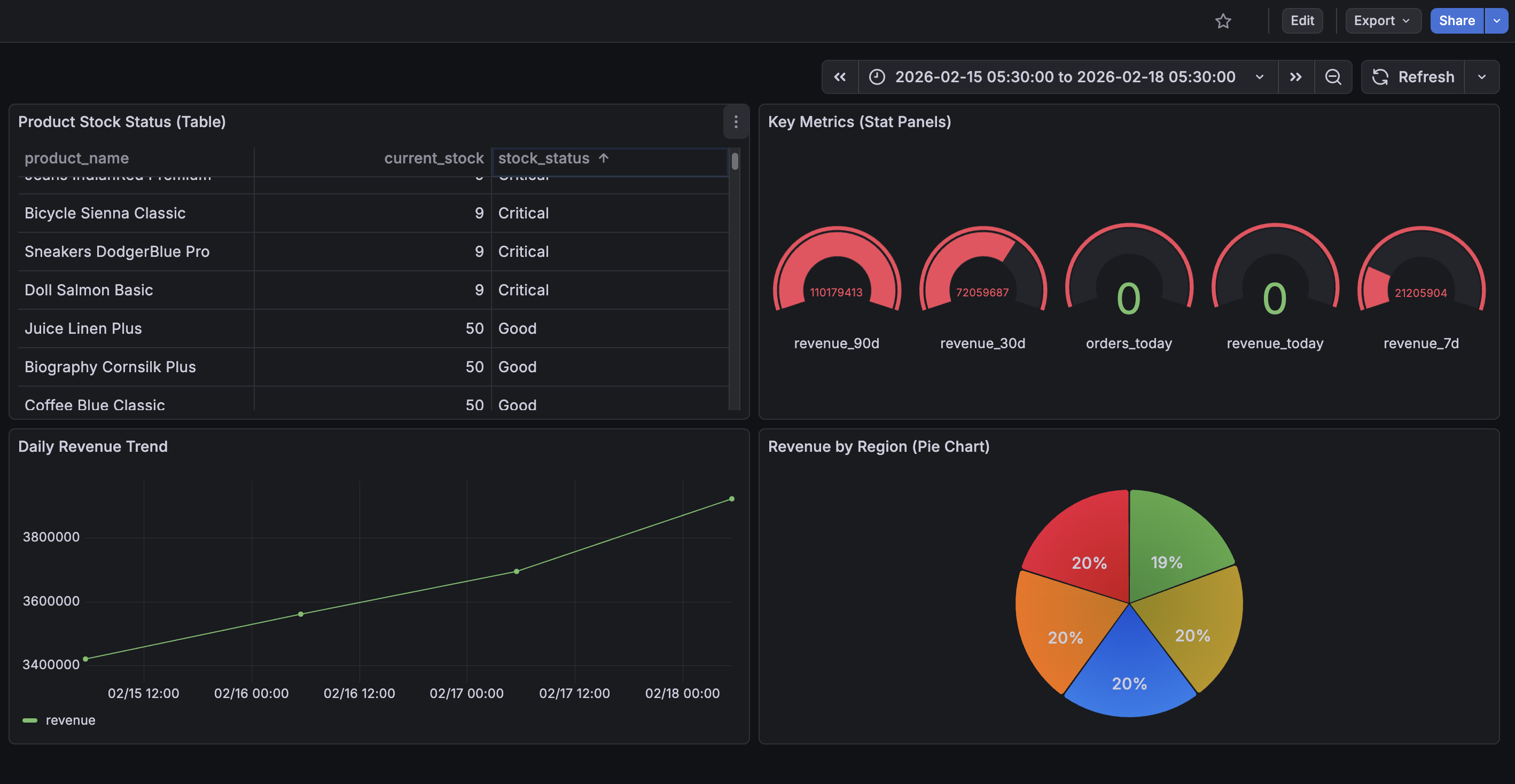
From this data, we want metrics like daily sales by region, revenue trends over 7/30/90 day windows, product performance and stock status, and order counts. These are the questions analytics teams ask daily, and this pipeline answers them automatically.

Medallion Architecture

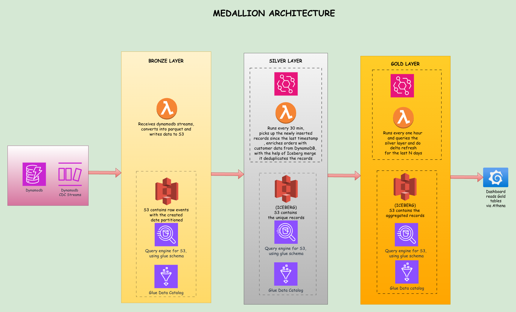
The medallion architecture organizes data into three layers: Bronze, Silver, and Gold. Each layer has a specific purpose and quality level. Think of it as a refinement process where raw materials get processed into finished goods.

Bronze Layer: Raw Data Ingestion

The Bronze layer captures data exactly as it arrives. When a record is inserted, modified, or removed in DynamoDB, the stream event triggers a Lambda function that writes the raw event to S3. Nothing is transformed or validated here. The goal is to land data quickly and preserve its original form for auditability.

Bronze data includes metadata like the event type (INSERT/MODIFY/REMOVE), the timestamp when the event occurred, and the source table name. This raw data acts as our system of record. If something goes wrong downstream, we can always go back to Bronze and reprocess.

Silver Layer: Cleaned and Enriched Data

The Silver layer is where we clean, deduplicate, and enrich the data. When an order arrives, it carries only a CustomerID. For analytics, we need to know which region that customer belongs to. The Silver Lambda reads Bronze data, looks up the customer's region from DynamoDB, and adds it to the order record.

This layer uses Apache Iceberg tables, which provide ACID transactions and in-place updates. When the same order arrives multiple times due to retries or updates, the MERGE operation keeps only the latest version without duplicates.

Gold Layer: Business-Ready Aggregates

The Gold layer contains pre-calculated metrics ready for dashboard consumption. Instead of running a complex aggregation on every dashboard load, we compute aggregates once per hour and store the results. When Grafana loads, it reads from these pre-computed tables, keeping queries fast and cheap.

The Gold layer includes daily_sales_by_region which aggregates orders by date and region, product_performance which shows stock levels and pricing, and key_metrics which contains revenue totals for different time windows. All three are Iceberg tables.

daily_sales_by_region uses a delta refresh strategy: only the last few days of data are recomputed on each run while historical aggregates are preserved. product_performance and key_metrics do a full replace on each run since they are small snapshot tables where every row can change.

Why This Layered Approach Works

Each layer has a single responsibility: Bronze for capture, Silver for transformation, Gold for presentation. When something breaks, you know exactly where to look. When requirements change, you modify one layer without affecting the others.

This separation also enables different latency tiers. Bronze lands data within one second of a DynamoDB write. Silver processes new Bronze files every 30 minutes. Gold publishes fresh aggregates every hour.

CDC Stream

Change Data Capture is the technique of recording data changes as they happen. DynamoDB Streams implements CDC by maintaining a time-ordered sequence of item-level modifications. When you insert, update, or delete a record, DynamoDB writes that change to the stream.

How DynamoDB Streams Work

Enabling streams with stream_view_type = "NEW_AND_OLD_IMAGES" means every write produces a stream record with the event type (INSERT, MODIFY, or REMOVE), the record's state before the change, and its state after. Stream records are retained for 24 hours and multiple consumers can read from the same stream independently.

The Data Lake: Storage and Query Layer

Once a Parquet file lands in S3, three AWS services work together to make it queryable with standard SQL.

S3 is the storage layer. It holds all Parquet files organized by layer, table name, and date partitions. S3 has no concept of tables or schemas; it just stores files.

Glue Catalog is the metadata layer. It stores table definitions including column names, data types, file format, and S3 location. Think of it as a phone book that maps logical table names to physical file locations.

Athena is the query engine. When you run a SQL query, Athena looks up the table definition in Glue Catalog, determines which S3 files to read, executes the query in parallel across those files, and returns results.

S3 Path Structure

The data lake follows a consistent folder structure:

s3://my-bucket/
├── bronze/
│   ├── orders-table/
│   │   └── year=2026/month=01/day=26/
│   │       ├── 20260126120530_a3f8b2c1.parquet
│   │       └── 20260126120530_7e2d4f09.parquet
│   ├── products-table/
│   └── customers-table/
├── silver/
│   ├── watermark.json            # Tracks last processed timestamp
│   ├── staging/                  # Temporary files (auto-cleaned after MERGE)
│   └── iceberg/
│       ├── orders/
│       │   ├── data/             # Parquet data files (managed by Iceberg)
│       │   └── metadata/         # Iceberg snapshots and manifests
│       ├── products/
│       └── customers/
└── gold/
    ├── daily_sales_by_region/
    │   ├── data/                 # Iceberg-managed data files
    │   └── metadata/             # Iceberg metadata
    ├── product_performance/
    └── key_metrics/

Bronze uses date partitioning in Hive style (year=2026/month=01/day=26). This enables partition pruning: when a query filters on WHERE year = '2026' AND month = '01', Athena skips all other prefixes instead of scanning the full table.

The Bronze Lambda writes each batch as a Parquet file rather than JSON or CSV. Parquet is a columnar format, so data is stored by column rather than by row. When Athena needs only three columns out of twenty, it reads just those three from disk. This directly reduces scanned data and cost, since Athena charges $5 per TB scanned. Parquet also uses Snappy compression, typically cutting file sizes by 70 to 80 percent compared to raw JSON, and it embeds schema information so Athena can infer structure without manual definition.

Table Types: Regular vs Iceberg

Notice that Bronze stores plain Parquet files while Silver and Gold have iceberg/ directories with data/ and metadata/ subdirectories. That reflects a fundamental difference in table type.

Bronze tables are regular external tables. Each Parquet file is immutable once written. Athena can read them but cannot update individual rows.

Silver and Gold use Apache Iceberg tables. Iceberg adds transactional capabilities on top of Parquet by maintaining metadata files that track which data files are current, which are superseded, and the full schema history. This enables two operations that plain Parquet cannot support.

The Silver layer needs MERGE. When you run MERGE INTO table USING source ON key WHEN MATCHED THEN UPDATE WHEN NOT MATCHED THEN INSERT, Iceberg determines which files to modify, writes updated versions, and atomically swaps the metadata pointer. Without Iceberg, you would delete and rewrite the entire table on every run.

The Gold layer needs row-level DELETE. Delta refresh works by deleting only the last N days of aggregates and inserting fresh ones, preserving historical data beyond that window. Without Iceberg, you would drop and recreate the entire table on every run, losing all historical aggregates.

Iceberg writes do accumulate snapshots over time. The implications of that and how to manage them are covered in Part 2 after the Silver and Gold Lambda implementations.

Terraform Setup

The entire infrastructure is defined in Terraform, organized into logical files based on resource type.

main.tf configures the Terraform backend and AWS provider. It sets up default tags applied to all resources, which helps with cost tracking and organization.

dynamodb.tf creates the three DynamoDB tables. Each table has streams enabled with NEW_AND_OLD_IMAGES, meaning DynamoDB captures both the before and after states of every change. Each table also has a Global Secondary Index for operational queries the application may need.

resource "aws_dynamodb_table" "orders" {
  name             = "${var.project_name}-orders-${var.environment}"
  billing_mode     = "PAY_PER_REQUEST"
  hash_key         = "OrderID"
  stream_enabled   = true
  stream_view_type = "NEW_AND_OLD_IMAGES"
  # ...
}

s3.tf creates two S3 buckets. The data lake bucket stores all Bronze, Silver, and Gold layer data. The Athena results bucket stores query output. Lifecycle policies transition older Bronze data to cheaper storage classes (Standard-IA after 90 days, Glacier after 180 days).

lambda.tf defines the three Lambda functions and their triggers. The Bronze Lambda is triggered by DynamoDB Streams via event source mappings. Silver and Gold are triggered by EventBridge schedule rules, with Silver running every 30 minutes and Gold running every hour.

# Silver runs every 30 minutes, scans for new Bronze files
resource "aws_cloudwatch_event_rule" "silver_processing_schedule" {
  name                = "${var.project_name}-silver-processing-${var.environment}"
  schedule_expression = "rate(30 minutes)"
}

# Gold runs on an hourly schedule
resource "aws_cloudwatch_event_rule" "gold_processing_schedule" {
  name                = "${var.project_name}-gold-processing-${var.environment}"
  schedule_expression = "rate(1 hour)"
}

glue.tf creates three Glue Catalog databases, one per layer. These are logical containers that group related tables. When Athena runs a query, it looks up table definitions from the Glue Catalog.

athena.tf creates the Athena workgroup with engine version 3, which supports Iceberg tables. The workgroup specifies a default output location for query results.

iam.tf defines IAM roles and policies for each Lambda following least-privilege. The Bronze Lambda needs permissions to read from DynamoDB Streams and write to S3. The Silver Lambda needs read/write/delete on S3, read from DynamoDB for customer lookups, Athena query execution, and Glue table management. The Gold Lambda needs the same S3 and Athena permissions. s3:DeleteObject is required for cleaning up temporary staging files after MERGE operations. Iceberg uses a copy-on-write strategy where old data files become orphaned rather than deleted, but the staging Parquet files that feed MERGE queries must be cleaned up explicitly.

tables.tf defines Bronze layer table schemas in the Glue Catalog with partition projection enabled. Silver and Gold tables are not defined here because Iceberg tables must be created by Athena's CREATE TABLE command to get proper metadata. Pre-creating them via Terraform causes cryptic errors.

To deploy, run terraform init followed by terraform apply. The deployment creates approximately 40 AWS resources and takes about 5 minutes.

Continue to Part 2 for Lambda implementations, data validation, Grafana setup, limitations, cost estimates, and conclusion.