
Building a Near Real-Time Analytics Pipeline: From DynamoDB to Grafana Dashboard
Part 2: Implementation, Dashboard, and Operations
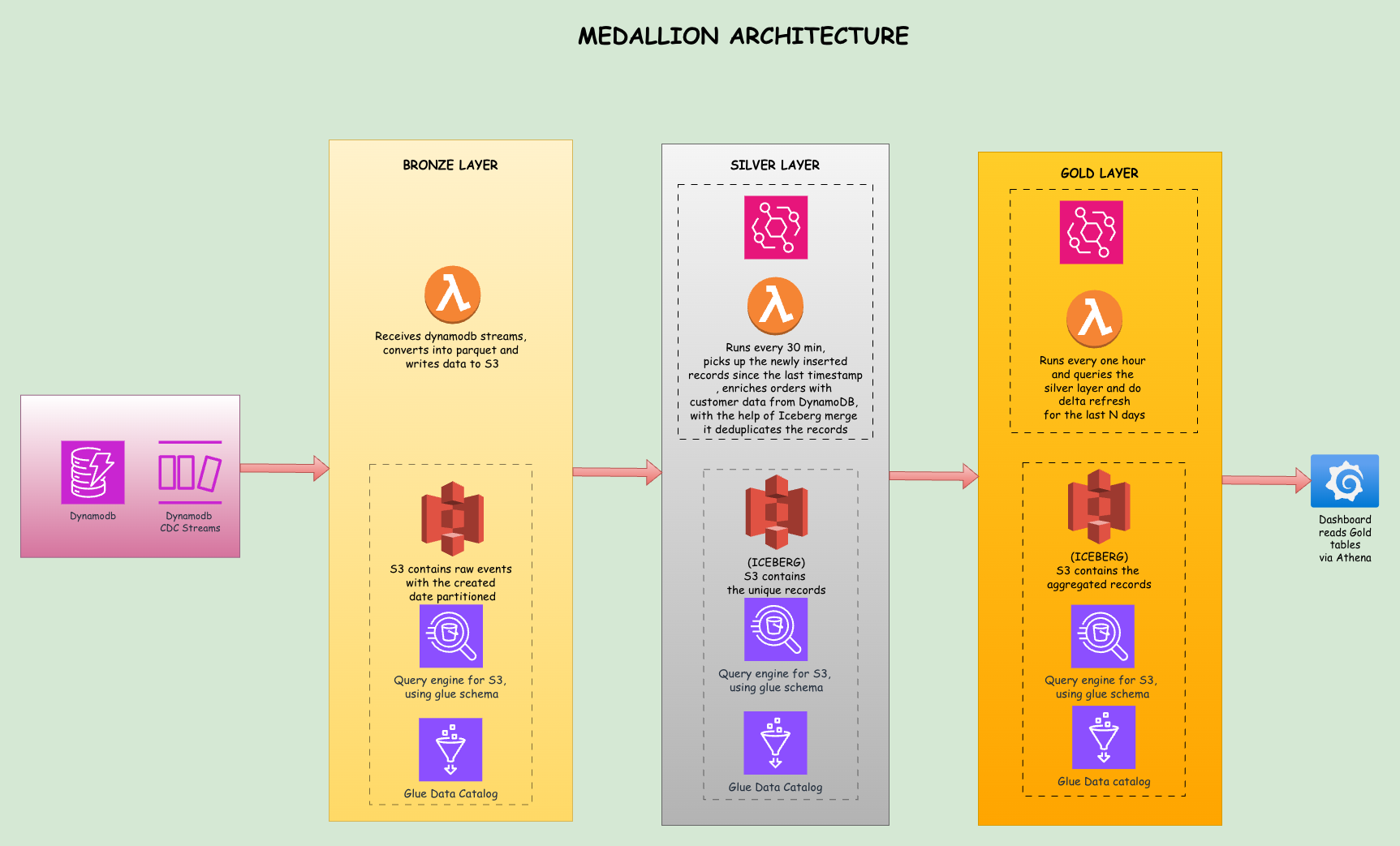
This is Part 2 of a two part series. Part 1 covered the problem, medallion architecture, CDC, the data lake storage and query layer, and Terraform setup. Part 2 covers Lambda implementations, data validation, Grafana setup, limitations, cost estimates, and conclusion.
The Bronze Lambda
When the Bronze Lambda receives a batch of stream records, it processes them into a simple format. Here is the core logic:
def lambda_handler(event, context):
    records = []

    for record in event['Records']:
        table_name = extract_table_name(record['eventSourceARN'])
        event_name = record['eventName']  # INSERT, MODIFY, REMOVE

        if event_name == 'REMOVE' or 'NewImage' not in record['dynamodb']:
            continue

        new_image = flatten_dynamodb_item(record['dynamodb']['NewImage'])

        records.append({
            '_event_name': event_name,
            '_event_timestamp': datetime.utcnow().isoformat(),
            '_table_name': table_name,
            **new_image
        })

    # Write to S3 as Parquet with date partitioning + UUID for uniqueness
    now = datetime.utcnow()
    batch_id = uuid.uuid4().hex[:8]
    s3_key = (f"bronze/{table_name}/year={now.year}/month={now.month:02d}"
              f"/day={now.day:02d}/{now.strftime('%Y%m%d%H%M%S')}_{batch_id}.parquet")

    table = pa.Table.from_pylist(records)
    buffer = io.BytesIO()
    pq.write_table(table, buffer, compression='snappy')

    s3_client.put_object(Bucket=S3_BUCKET, Key=s3_key, Body=buffer.getvalue())
The Lambda extracts the table name from the stream ARN, flattens the DynamoDB item format (converting {"S": "hello"} to plain "hello"), adds metadata fields prefixed with underscore, and writes everything to S3 as a Parquet file.
Notice the batch_id UUID suffix in the filename. With batch_size=100, a burst of 1000 inserts produces roughly 10 concurrent Lambda invocations. Without the UUID, two invocations finishing in the same second would write to the same S3 key (e.g., 20260216153042.parquet), and S3's last-writer-wins behavior would silently overwrite one batch. The UUID ensures every file is unique regardless of timing.
How the Silver Lambda Works
The Silver Lambda runs on a 30-minute schedule via EventBridge. Instead of reacting to individual file arrivals, it uses a watermark: a small JSON file stored in S3 (silver/watermark.json) that records the timestamp of the last successful run. On each invocation, the Lambda:
- Reads the watermark to determine when it last ran
- Scans all Bronze prefixes for Parquet files with
LastModifiednewer than the watermark - Reads all new files into memory as a single batch
- Transforms and enriches the records (e.g., adding customer region to orders)
- Writes a staging Parquet file to a temporary S3 location with a UUID-based path
- Creates a temporary external table in Athena pointing at the staging file
- Runs a MERGE INTO against the Iceberg table to upsert records
- Cleans up the temp table and staging file
- Saves the new watermark so the next run picks up from where this one left off
A scheduled approach is necessary here. When a burst of Bronze files lands simultaneously (say, 10 files from a batch insert), S3 notifications would trigger 10 concurrent Silver invocations all trying to MERGE into the same Iceberg table. Iceberg requires exclusive writes, so concurrent MERGEs cause ICEBERG_COMMIT_ERROR failures. A scheduled Lambda serializes all processing into a single invocation, eliminating concurrency conflicts entirely.
What if the watermark gets corrupted or deleted? If watermark.json is missing or unreadable, the Lambda defaults to a timestamp 24 hours in the past, causing it to scan and reprocess all recent Bronze files. Since MERGE is idempotent (matching records get updated, not duplicated), reprocessing produces the correct result without data corruption. The watermark is only saved after all tables are processed successfully, so a mid-run crash causes the next invocation to replay from the last good watermark with no silent data loss.
Here is the core enrichment logic:
def enrich_order_data(order):
    """Enrich orders with customer data from DynamoDB"""
    customer_id = order.get('CustomerID')
    if not customer_id:
        return order

    table = dynamodb.Table(CUSTOMERS_TABLE)
    try:
        response = table.get_item(Key={'CustomerID': customer_id})
        if 'Item' in response:
            customer = response['Item']
            order['customer_name'] = customer.get('Name', '')
            order['customer_region'] = customer.get('Region', '')
    except Exception as e:
        print(f"  Warning: Could not enrich customer {customer_id}: {e}")

    return order
The MERGE query handles deduplication: if an order with the same OrderID already exists it gets updated, otherwise it gets inserted:
MERGE INTO orders_enriched t
USING temp_staging_table s
ON t.orderid = s.orderid
WHEN MATCHED THEN UPDATE SET
    customerid = s.customerid,
    orderdate = s.orderdate,
    totalamount = s.totalamount,
    customer_name = s.customer_name,
    customer_region = s.customer_region,
    event_timestamp = s.event_timestamp,
    processing_timestamp = s.processing_timestamp
WHEN NOT MATCHED THEN INSERT (
    orderid, customerid, orderdate, totalamount,
    customer_name, customer_region, event_timestamp,
    processing_timestamp
) VALUES (
    s.orderid, s.customerid, s.orderdate, s.totalamount,
    s.customer_name, s.customer_region, s.event_timestamp,
    s.processing_timestamp
)
Before running the MERGE, the Lambda also deduplicates within the batch. If the same primary key appears multiple times across Bronze files (due to rapid updates), only the latest version is kept. This prevents MERGE_TARGET_ROW_MULTIPLE_MATCHES errors.
Why Silver Needs a Staging Directory
You might wonder why we write to a staging file at all, rather than having Athena read Bronze directly.
The reason is that enrichment happens in Python, not SQL. When the Silver Lambda processes orders, it calls DynamoDB for each record to fetch the customer's name and region. Athena cannot call DynamoDB mid-query. So once Python has enriched the data in memory, it needs to materialize those enriched records back to S3 as a Parquet file (the staging file), create a temporary Athena table pointing at it, and then run the MERGE.
An alternative design would skip the DynamoDB lookup entirely and JOIN Bronze orders with Silver customers inside a single Athena SQL query. But that introduces an ordering dependency (customers must be processed before orders on every run) and sacrifices per-record enrichment logic in Python.
The Gold Lambda, by contrast, does not use staging at all. It reads directly from Silver Iceberg tables and writes to Gold Iceberg tables using pure SQL within Athena.
After a successful MERGE, the Silver Lambda deletes the staging file in a finally block. If the Lambda times out before cleanup, orphaned staging files may remain in S3. They do not affect correctness (each run writes to a unique UUID-based path), but adding an S3 lifecycle rule to auto-expire files under silver/staging/ after a few days is a good safety net.
Iceberg Snapshot Management
The Silver Lambda runs a MERGE every 30 minutes and the Gold Lambda runs DELETE and INSERT every hour. Both operations create Iceberg snapshots. Before looking at the Gold Lambda, it is worth understanding what accumulates and how to clean it up.
Every MERGE, INSERT, or DELETE against an Iceberg table creates a new snapshot. A snapshot is a pointer to the set of data files that represent the table at that point in time. Iceberg uses a copy-on-write strategy: when a MERGE updates 5 records in a Parquet file containing 1000 records, Iceberg writes a new file with all 1000 records (5 updated, 995 unchanged), and the new snapshot points to the new file. The old file is not deleted; it becomes an "orphan" no longer referenced by any current snapshot.
Over time, this creates two problems: snapshot accumulation (metadata grows with every write) and orphaned files (old data files that waste storage). In production, address these with:
- Snapshot expiration:
ALTER TABLE ... EXECUTE expire_snapshots(retention_threshold => '7d')removes snapshots older than the threshold, keeping metadata lean. - Orphan file removal: After expiring snapshots, clean up their unreferenced data files with
ALTER TABLE ... EXECUTE remove_orphan_files(retention_threshold => '7d'). - Compaction: Frequent small writes (like the 30-minute MERGE) create many small files.
ALTER TABLE ... EXECUTE optimizerewrites them into fewer, larger files, improving query performance.
At this pipeline's scale, snapshot growth is modest. A weekly or monthly cleanup job is sufficient. At larger scales, these operations become critical for keeping costs and query times under control.
How the Gold Lambda Works
The Gold Lambda runs hourly and uses Iceberg tables with delta refresh. Instead of dropping and recreating tables on every run, it deletes only the last N days of data and re-inserts fresh aggregates for that window. Historical data beyond the refresh window is preserved untouched.
This is the key advantage of Iceberg in the Gold layer: row-level DELETE on S3 data, which plain Parquet tables cannot do.
The Gold tables are created as Iceberg tables on the first run:
CREATE TABLE daily_sales_by_region (
    order_date DATE,
    region STRING,
    order_count BIGINT,
    total_revenue DOUBLE,
    avg_order_value DOUBLE,
    unique_customers BIGINT,
    computed_at TIMESTAMP
)
LOCATION 's3://bucket/gold/daily_sales_by_region/'
TBLPROPERTIES ('table_type'='ICEBERG')
On each subsequent run, the delta refresh is a two-step process: delete stale data, then insert fresh:
-- Step 1: Remove stale aggregates for the refresh window
DELETE FROM daily_sales_by_region
WHERE order_date >= CURRENT_DATE - INTERVAL '3' DAY

-- Step 2: Insert fresh aggregates from Silver
INSERT INTO daily_sales_by_region
SELECT
    CAST(date_parse(orderdate, '%Y-%m-%d %H:%i:%s') AS DATE) as order_date,
    customer_region as region,
    COUNT(*) as order_count,
    SUM(totalamount) as total_revenue,
    AVG(totalamount) as avg_order_value,
    COUNT(DISTINCT customerid) as unique_customers,
    CAST(CURRENT_TIMESTAMP AS TIMESTAMP) as computed_at
FROM "{SILVER_DB}".orders_enriched
WHERE CAST(date_parse(orderdate, '%Y-%m-%d %H:%i:%s') AS DATE)
      >= CURRENT_DATE - INTERVAL '3' DAY
    AND customer_region IS NOT NULL
GROUP BY CAST(date_parse(orderdate, '%Y-%m-%d %H:%i:%s') AS DATE),
         customer_region
Note: {SILVER_DB} is a Python f-string variable that resolves to the Silver Glue database name (e.g., ecommerce-analytics-silver-dev). Since it contains hyphens, double-quoting is required in Athena SQL.
The refresh window (default: 3 days) is configurable via the REFRESH_DAYS environment variable. For product_performance and key_metrics, we do a full replace (delete all rows and insert fresh), since these are small snapshot tables where preserving history does not apply.
Why Delta Refresh Matters
Consider a dashboard showing 90 days of daily revenue trends. With a full refresh, the Gold Lambda would re-aggregate all 90 days of Silver data on every hourly run, even though only today's numbers changed. With delta refresh, it recomputes only the last 3 days and leaves the other 87 untouched. As data grows, this difference compounds: the Athena query scans less data (cheaper), runs faster, and the Lambda stays well within its 15-minute timeout.
The 3-day window accounts for late-arriving data and corrections. If an order from yesterday gets modified today, Silver updates it via MERGE, and the next Gold refresh picks up the corrected aggregate.
Deployment
Before the pipeline runs you need two things: deployment packages for the Lambda functions and the Terraform apply. Prerequisites are Python 3.11, Terraform 1.5+, and an AWS CLI profile with permission to create IAM roles, Lambda functions, DynamoDB tables, S3 buckets, and Athena workgroups.
Build the Lambda packages. Each function packages only its handler.py. pyarrow lives in a shared Lambda layer so the function zips stay small. A build script handles everything, including downloading a Linux-compatible pyarrow wheel (necessary even on macOS since Lambda runs on Linux):
chmod +x scripts/build_lambda.sh
./scripts/build_lambda.sh
This produces lambda/layers/python_deps.zip and a deployment.zip in each of the bronze/, silver/, and gold/ directories.
Configure and apply Terraform. Copy the example vars file, update if needed, and apply:
cp terraform/terraform.tfvars.example terraform/terraform.tfvars
# edit aws_region, project_name, s3_bucket_prefix as needed

cd terraform
terraform init
terraform apply
S3 bucket names must be globally unique. If the apply fails on a bucket conflict, change s3_bucket_prefix in terraform.tfvars. The full apply creates roughly 38 resources and takes about 5 minutes.
Data Validation
Seed DynamoDB, trigger each Lambda manually, and confirm row counts match at each layer.
Seed the data. Orders depend on existing customers and products, so generate them in this order:
python scripts/generate_data.py \
  --customers-table ecommerce-analytics-customers-dev \
  --products-table ecommerce-analytics-products-dev \
  --orders-table ecommerce-analytics-orders-dev \
  --num-customers 100 \
  --num-products 50 \
  --num-orders 500
DynamoDB Streams fire as records are written and the Bronze Lambda processes them within seconds. Check that Parquet files appeared:
aws s3 ls s3://ddb-analytics-ecommerce-analytics-<account-id>/bronze/ --recursive | head -20Trigger Silver and verify counts. Rather than waiting 30 minutes for the schedule, invoke it directly:
aws lambda invoke \
  --function-name ecommerce-analytics-silver-processor-dev \
  --payload '{}' /tmp/silver-out.json && cat /tmp/silver-out.json
Then confirm the Silver Iceberg tables have the expected rows in Athena. The count in orders_enriched should match the 500 orders you seeded:
SELECT COUNT(*) FROM "ecommerce-analytics-silver-dev".orders_enriched;
-- expected: 500
Trigger Gold and verify aggregates.
aws lambda invoke \
  --function-name ecommerce-analytics-gold-processor-dev \
  --payload '{}' /tmp/gold-out.json && cat /tmp/gold-out.json
SELECT * FROM "ecommerce-analytics-gold-dev".daily_sales_by_region
ORDER BY order_date DESC LIMIT 10;Rows grouped by date and region with non-zero revenue confirm the full pipeline is working.
Grafana Setup
Grafana connects to Athena as a data source and visualizes the Gold layer tables.
Step 1: Configure the Athena Data Source
The datasource is configured via provisioning YAML at grafana/provisioning/datasources/athena.yml:
apiVersion: 1
datasources:
  - name: Athena - E-commerce Analytics
    type: grafana-athena-datasource
    access: proxy
    isDefault: true
    jsonData:
      authType: keys
      defaultRegion: us-east-1
      catalog: AwsDataCatalog
      database: ecommerce-analytics-gold-dev
      workgroup: ecommerce-analytics-workgroup-dev
      outputLocation: s3://your-athena-results-bucket/grafana-queries/
    secureJsonData:
      accessKey: ${AWS_ACCESS_KEY}
      secretKey: ${AWS_SECRET_KEY}
    editable: true
Step 2: Create Environment File
Create a .env file with your AWS credentials and add it to .gitignore:
AWS_ACCESS_KEY=your-access-key
AWS_SECRET_KEY=your-secret-key
Step 3: Start Grafana
docker-compose up -dAccess Grafana at http://localhost:3000 with default credentials admin/admin.
Step 4: Create Dashboard Panels
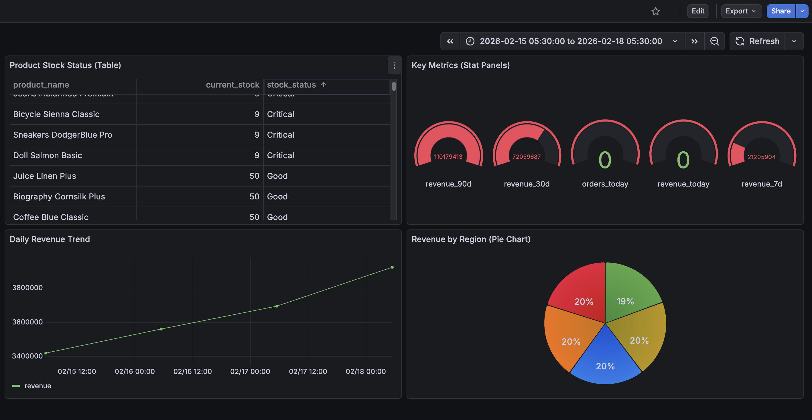
Navigate to Dashboards, create a new dashboard, and add visualizations using the Athena data source with these queries:
Revenue by Region (Pie Chart):
SELECT region, SUM(total_revenue) as revenue
FROM daily_sales_by_region
WHERE order_date >= CURRENT_DATE - INTERVAL '30' DAY
GROUP BY region
Daily Revenue Trend (Time Series):
SELECT order_date as time, SUM(total_revenue) as revenue
FROM daily_sales_by_region
WHERE order_date >= CURRENT_DATE - INTERVAL '30' DAY
GROUP BY order_date
ORDER BY order_date
Key Metrics (Stat Panels):
SELECT metric_name, metric_value
FROM key_metrics
WHERE metric_name = 'revenue_30d'
Product Stock Status (Table):
SELECT product_name, current_stock, stock_status
FROM product_performance
ORDER BY current_stock ASC
Set the dashboard auto-refresh to 5 to 10 minutes to show updated data as the pipeline runs.
Limitations
This architecture works well for small to medium workloads, but there are thresholds where you should consider alternatives.
Lambda Execution Time: AWS Lambda has a maximum timeout of 15 minutes. The Silver Lambda runs Athena queries and waits for completion, which can take several minutes for large MERGE operations. If processing exceeds this limit, consider moving to AWS Glue ETL jobs or EMR Serverless, which have no execution time ceiling.
DynamoDB Streams Retention: Streams retain data for only 24 hours. If your Lambda fails for an extended period, you will miss events. For mission-critical pipelines, consider adding a dead-letter queue or using Kinesis Data Streams as an intermediate buffer.
Athena Query Concurrency: Athena has default concurrency limits of 20 to 25 queries per account per region. Since Silver and Gold Lambdas run on schedules rather than event-driven triggers, concurrency is well-controlled. However, if you add more tables or run ad-hoc queries alongside the pipeline, you may approach these limits.
When to Graduate:
- Kinesis Data Firehose: When DynamoDB Streams' 24-hour retention becomes a risk. Firehose can sit between DynamoDB Streams and S3, providing automatic batching, buffering, and longer delivery guarantees. If the Bronze Lambda fails for hours, Firehose continues buffering records. It also supports native Parquet delivery to S3, which could replace the Bronze Lambda entirely.
- PySpark on EMR/Glue: When daily volume exceeds a few million records or Silver processing consistently takes over 10 minutes.
- Apache Airflow (or MWAA): When you need complex step dependencies, sophisticated retry logic, or visual monitoring of pipeline runs.
- Databricks: When you need advanced features like Z-ordering and bloom filters, or your team prefers notebooks over Lambda code.
The architecture naturally evolves. You can replace the Silver Lambda with a Glue PySpark job while keeping everything else intact. The medallion pattern is the foundation; the specific tools are interchangeable.
Cost Estimates
Every component in this architecture is pay-per-use. Here is what to expect at different scales:
Low Volume (~1K orders/day, dev/staging)
| Service | Usage | Estimated Monthly Cost |
|---|---|---|
| DynamoDB (on-demand) | ~30K writes/month + streams | ~$1–2 |
| Lambda (3 functions) | Bronze: ~30K invocations; Silver: ~1,440; Gold: ~720 | ~$0–1 (free tier covers most) |
| S3 storage | ~100 MB across all layers | ~$0.01 |
| Athena queries | ~2,160 queries/month (Silver + Gold), scanning <1 GB total | ~$0.01–0.05 |
| Glue Catalog | 3 databases, ~10 tables | Free (first million objects) |
| EventBridge | ~2,160 invocations/month | Free (first million events) |
| Grafana | Self-hosted via Docker (local) | Free |
| Total | ~$2–5/month |
Medium Volume (~50K orders/day, production)
| Service | Usage | Estimated Monthly Cost |
|---|---|---|
| DynamoDB (on-demand) | ~1.5M writes/month + streams | ~$20–30 |
| Lambda | Bronze: ~15K invocations; Silver/Gold: same schedule | ~$2–5 |
| S3 storage | ~5–10 GB across all layers | ~$0.25–0.50 |
| Athena queries | Same query count, scanning ~10–50 GB/month | ~$0.50–2.50 |
| Grafana | Self-hosted on EC2 (t3.small) or ECS | ~$15–20 |
| Total | ~$40–60/month |
Grafana Hosting Options
In this blog, we run Grafana locally via Docker Compose at zero cost. For production, you have a few options:
- Self-hosted on EC2/ECS: Run the Grafana Docker container on a small instance (t3.small is roughly $15/month). You manage updates and availability.
- Grafana Cloud (free tier): Up to 3 users and 14 days of retention. Just configure the Athena data source plugin and point it at your AWS account.
- Grafana Cloud (paid): Starts at $55/month per stack for teams, including alerting, SLOs, and longer retention.
- Amazon Managed Grafana: AWS-native at roughly $9/editor/month. Integrates with IAM for Athena access so you do not need to pass AWS keys via environment variables.
What Drives Costs Up
- Athena scans: Athena charges $5/TB scanned. Parquet and partition pruning keep this low, but unpartitioned Gold tables or
SELECT *queries can inflate costs. - DynamoDB writes: On-demand mode at high volume. Provisioned capacity with auto-scaling is cheaper for predictable workloads.
- Lambda duration: The Silver Lambda waits for Athena queries; slow MERGEs on large tables add up in duration charges.
- S3 storage: Iceberg's copy-on-write creates orphaned files. Without periodic cleanup (see Iceberg Snapshot Management above), storage grows faster than expected.
- Grafana dashboard queries: Each panel refresh triggers an Athena query. With 5 panels auto-refreshing every 5 minutes, that is 1,440 queries per day. Querying pre-computed Gold tables keeps scan sizes small, but be mindful of refresh intervals.
The pipeline comfortably runs under $5/month for development (with Grafana running locally) and under $60/month for moderate production workloads including a hosted Grafana instance, a fraction of what a dedicated EMR cluster or Redshift instance would cost.
Conclusion
We built a complete near real-time analytics pipeline that takes data from DynamoDB, processes it through Bronze, Silver, and Gold layers, and presents it in Grafana dashboards. The pipeline handles deduplication using Iceberg MERGE operations, enriches data by joining across tables in Python, and pre-computes aggregates for fast dashboard queries. The entire infrastructure is defined in Terraform and runs serverlessly with no clusters to manage.
The key insights: separate concerns into distinct layers, use the right table format for each layer's needs (regular Parquet for immutable data, Iceberg for mutable data), pre-compute aggregates rather than running expensive queries at dashboard load time, and keep transformations simple enough to fit within Lambda's execution limits. When scale demands it, individual components swap out cleanly while the rest of the pipeline stays unchanged.
The complete source code is available on GitHub: dynamodb-to-grafana